Potential Improvements in Dispersion Modelling with WRF: Application to the Collie airshed in Western Australia

The Challenge

USEPA recommended dispersion models, i.e. AERMOD [1, 2] and CALPUFF [3], do not perform well in simulating the observed ground level concentrations of SO2 in the Collie airshed. In both models, parameters characterising the dispersion are related to the turbulence of the planetary boundary layer by the Monin-Obukhov stability theory [4, 5]. Plume models are known to produce inaccurate results at low wind speeds, since the fundamental assumption that downwind dispersion is negligible is not justified in this limit.
Alternatively, The Air Pollution Model (TAPM) developed by CSIRO programs [6] provide a time dependent description of air pollution dispersion by numerical solution of the advection dispersion equation. The prognostic meteorology capability of TAPM is often used to calculate the meteorological parameters required by simpler models in situations where suitable data are lacking. For the Collie region, numerical simulations by TAPM overestimate concentrations by a factor of about 1.5.
These pollution dispersion models rely for their parameterization on accurate meteorological data. For this purpose, we used the WRF model [7], which is currently regarded as one of the leading publicly available numerical weather prediction systems. WRF is a numerical model that essentially solves the compressible, non-hydrostatic Euler equations at each grid-point. It is under continuous development by a large scientific community. During model set up and optimisation, our team encountered several challenges, including:
• Model performance with default parametrisation is not satisfactory;
• Model run takes a long time for large airsheds like Collie airshed;
• The WRF model runs became unstable after the operating system upgrade earlier in 2018;
• The WRF model runs became unstable at the 6th grid (most inner grid). The calculation has encountered negative time steps as a result of a bug in WRF version 3.8.1 (fixed in WRF version 3.9.1) which resulted in the termination of the model simulations; and
• The representation of nocturnal low level atmospheric jets was not satisfactory.
The configuration of WRF contains hundreds of options, including boundary layer schemes, and other switches. The application of WRF is very flexible; however, optimisation of the configuration can be expensive in terms of time and computation on standard computers.

The Solution

Initially, three simulations were conducted for the year 1998 as follows:
• WRF with land surface data and topography data provided with WRF version 3.8.
• The land use and topography data were updated using Australian specific databases and topography.
• The topo_winds parameterisation was activated as this has been shown [8] to improve wind speed estimation produced by WRF east of the Darling Escarpment.
The modelled results are acceptable but with room for improvement. In order to improve the model performance, it is required to conduct multiple model runs. Some of the identified solutions for our challenges are:
• Upgrade WRF version from v3.8.1 to v3.9.1 to resolve the negative time step issue in the most inner grid;
• Enable adaptive time step to stabilise the model runs;
• Sensitivity analysis on mixing parameters and increase roughness length to improve the wind speed representation;
• Sensitivity analysis on various boundary layer schemes with different turbulence closures to improve the overall model performance; and
• Enable 2nd to 3rd grid nudging to improve overall model performance.
The architecture of the WRF model is designed for implementation on multi-processor machines. The code is mostly Fortran and is designed to run with distributed (MPI) or shared memory architecture (OpenMP), or a hybrid of the two.

The Outcome

The access to the Pawsey Magnus supercomputer allowed this project to run many high-resolution scenarios within a manageable time. This allows us to test the most potential solutions for our challenges. As a result, the model performance has improved significantly.
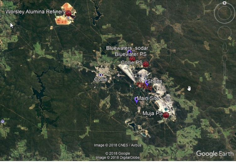
By writing script to automate the scenario runs in multiple threads and cores, we are able to conduct sensitivity analysis of various model configurations. The simulations conducted in 2017 and 2018 focussed on firstly optimising the model configuration and then comparing modelled and observed wind speed and direction for legacy observations from 1998 as well as recent observations in 2018. Figure 1 shows the Collie Region and the location of the Shotts meteorological monitoring station used to compare the model results.
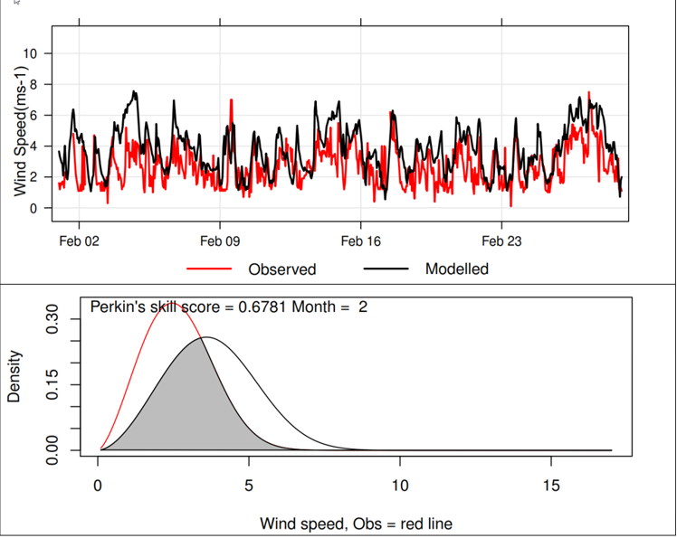
Analysis was undertaken using the open sourced National Centre for Atmospheric Research Command language (NCL) and R which are both available at Pawsey Magnus supercomputer. Model performance is measured based on the Perkins skill score (Perkins et al., 2007) [9] which compares the observed and modelled probability density functions. We have modified this by fitting the wind speed as well as wind direction data to a Weibull distribution before calculating the PDF.
The results for February 1998 are provided in Figures 2 to 4. From Figure 2, WRF demonstrates a general over prediction of wind speed. Using the updated land use and topography data in Figure 3 produces a slight change in the modelled winds. We have not yet tested the statistical significance of this difference of the modelled winds.
Using the improved parameterisation of larger scale topographic drag on local scale winds has made an improvement to the wind speed distribution from the model calculations. The mean wind is much closer to observed mean, but now appears to be under-estimating observed high winds (Perkins skill score: 0.64 – 0.79).
As part of the Collie Air shed study additional SO2 and meteorological monitoring data has been available from August 2017. These additional sites included a sodar (which measures wind speed at multiple heights) at the Blue Waters (site BWS) and an 80 m tower and RASS temperature and wind speed profiler (site MAI). We focused on analysis of model performance for March 1-15 2018 and extended the analysis to multiple heights. Figure 5 provides the modelled and compared wind speed for this period. An interesting feature of this period is the presence of strong night-time winds (nocturnal jets). These are evident at both 80m and 250m. The model over represents these nocturnal jets; particularly at 250m.
WRF provides several boundary layer schemes as well as roughness length parametrisation. Simulations were also extended to test whether one of these alternative boundary layer parameterisations which include use calculation of sub grid scale turbulent kinetic energy (TKE) to improve transfer of momentum fluxes closer to the surface and reduce the strength of the low level jets. The model performance has been improved significantly by switching from Yonsei University Scheme (YSU) scheme [10] to the Mellor–Yamada–Janjic (MYJ) scheme [11] (see Figure 6). This is a significant finding with implications for potential air quality uses in the South west of Western Australia as most simulations that we are aware of tend to use the YSU scheme by default. The next stage would be to extend the simulations to a full year to assess boundary layer performance over a greater range of conditions.

Without the Pawsey Magnus supercomputer and the assistance of the staff, optimising the model performance for the whole Collie air shed would likely be impossible

List of Publications

References
[1] Alan J. Cimorelli, Steven G. Perry, Akula Venkatram, Jeffrey C. Weil, Robert J. Paine, Robert B. Wilson, Russell F. Lee, Warren D. Peters, and Roger W. Brode. “AERMOD: A dispersion model for industrial source applications. Part I: General model formulation and boundary layer characterization,” Journal of Applied Meteorology, 44: 682-693 (2005).
[2] Steven G. Perry, Alan J. Cimorelli, Robert J. Paine, Roger W. Brode, Jeffrey C. Weil, Akula Venkatram, Robert B. Wilson, Russell F. Lee, and Warren D. Peters. “AERMOD: A dispersion model for industrial source applications. Part II: Model performance against 17 field study databases,” Journal of Applied Meteorology, 44: 694-708 (2005).
[3] Joseph S. Scire, David G. Strimaitis, and Robert J. Yamartino. “A User’s Guide for the CALPUFF Dispersion Model (Version 5),” Concord, MA: Earth Tech Inc. (2000).
[4] A.S. Monin and A.M. Obukhov. “Fundamental laws of turbulent mixing in the ground layer of the atmosphere,” Trudy Geofizicheskogo Instituta Akademii Nauk SSSR, 24 (151): 163-187 (1954).
[5] A.M. Obukhov. “Turbulence in an atmosphere with a non-uniform temperature,” Boundary Layer Meteorology, 2: 7-29 (1971).
[6] Peter Hurley. “TAPM v4. Part 1: Technical Description”. CSIRO Marine and Atmospheric Research Paper No. 25 (2008).
[7] J. Michalakes, S. Chen, J. Dudhia, L. Hart, J. Klemp, J. Middlecoff, and W. Skamarock. “Development of a Next Generation Regional Weather Research and Forecast Model,” in Developments in Teracomputing: Proceedings of the Ninth ECMWF Workshop on the Use of High Performance Computing in Meteorology. Eds. Walter Zwieflhofer and Norbert Kreitz. World Scientific, Singapore. pp. 269-276 (2001).
[8] Rye. P. “Getting the Most out of WRF” Air Quality and Climate Change, 50: 29-32 (2016).
[9] Perkins. S.E., Pitman. A.J., Holbrook, N.J., and McAneney, J. Evaluation of the AR4 Climate Models’ Simulated Daily Maximum Temperature, Minimum Temperature, and Precipitation over Australia Using Probability Density Functions. Journal of Climate 20 (2007).
[10] Hong, Song–You, Yign Noh, Jimy Dudhia. A new vertical diffusion package with an explicit treatment of entrainment processes. Mon. Wea. Rev., 134, 2318–2341 (2006).
[11] Janjic, Zavisa I. The Step–Mountain Eta Coordinate Model: Further developments of the convection, viscous sublayer, and turbulence closure schemes. Mon. Wea. Rev., 122, 927–945 (1994).